
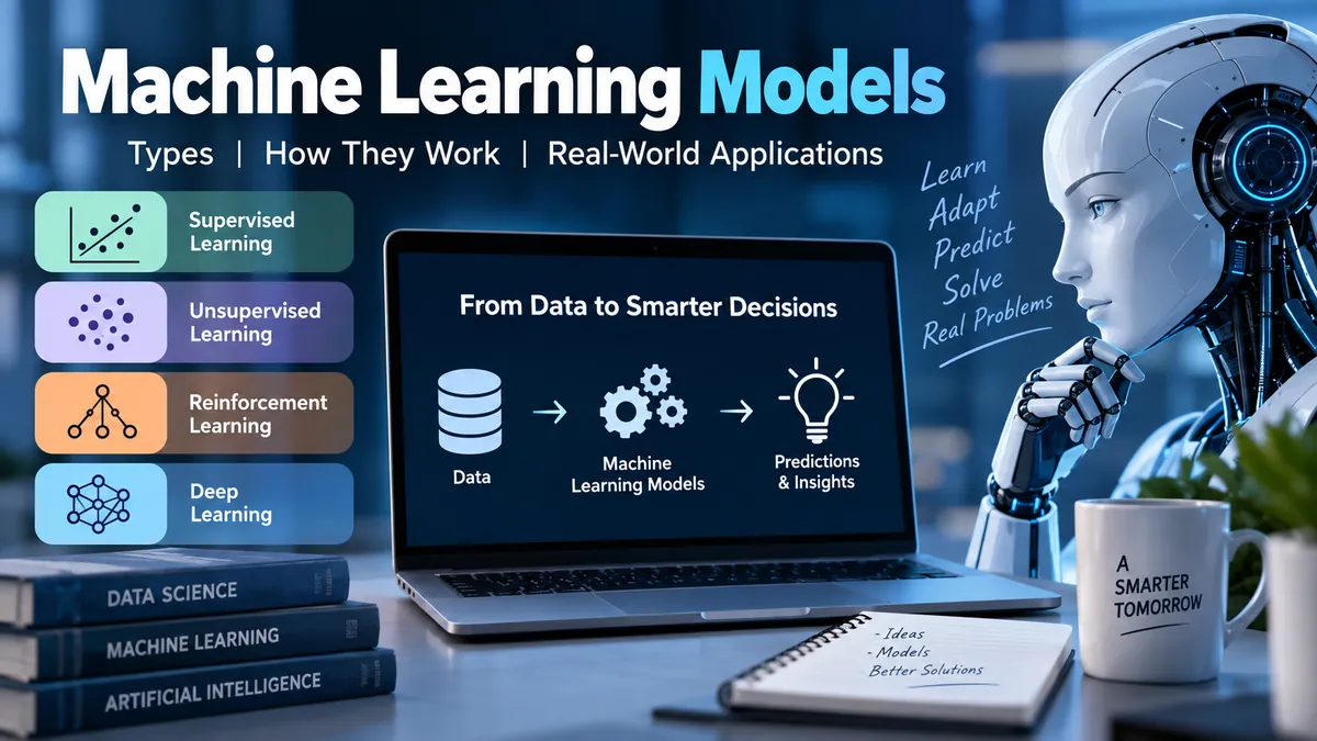

Machine learning models sit behind many systems people use every day, from spam filters and recommendation engines to fraud detection, forecasting, computer vision, and generative AI. Yet the term “model” is often mixed up with algorithms, artificial intelligence, and deep learning.
Machine learning models are trained mathematical or computational systems that learn patterns from data and use those patterns to make predictions, classifications, decisions, or discover structure in new data. They are created by applying machine learning algorithms to training data and adjusting model parameters until useful patterns generalize beyond the training examples.
Understanding the different models—and knowing when each one makes sense—is one of the foundations of practical machine learning.
What Are Machine Learning Models?
A machine learning model is the result of training a mathematical framework on data so that it can recognize relationships and produce useful outputs for previously unseen inputs.
Consider an email spam detector.
Instead of programming thousands of rigid rules such as “if an email contains this particular phrase, mark it as spam,” developers can provide examples of emails labeled spam and not spam. A learning algorithm identifies patterns associated with those labels.
Once training is complete, the resulting model can estimate whether a new email belongs to the spam or non-spam class.
This ability to generalize from examples distinguishes machine learning from traditional rule-based programming.
Machine learning is a subset of artificial intelligence (AI), and it now underpins systems ranging from forecasting applications and autonomous technologies to large language models (LLMs).
Machine Learning Model vs. Algorithm
The words model and algorithm are frequently used as though they mean the same thing, but there is an important distinction.
| Term | Meaning | Example |
|---|---|---|
| Algorithm | A procedure used to learn patterns from data | Decision tree algorithm |
| Model | The trained system produced by applying an algorithm to data | A trained credit-risk decision tree |
| Parameters | Values learned during training | Regression coefficients |
| Hyperparameters | Settings chosen before or during model training | Tree depth, learning rate |
| Prediction | Output generated from new input | “Fraud probability: 92%” |
Put simply:
Algorithm + training data + learning process → trained model
IBM similarly distinguishes algorithms as procedures from models as systems produced by applying those procedures to data.
This distinction becomes useful when comparing different machine learning techniques.
Main Types of Machine Learning Models
Machine learning methods are generally organized around three fundamental learning paradigms: supervised learning, unsupervised learning, and reinforcement learning. Modern workflows can also use semi-supervised and self-supervised approaches or combine multiple paradigms.
| Learning Type | Training Signal | Typical Goal | Example |
|---|---|---|---|
| Supervised | Labeled examples | Predict known targets | Fraud detection |
| Unsupervised | Unlabeled data | Discover hidden structure | Customer segmentation |
| Semi-supervised | Small labeled + large unlabeled dataset | Improve prediction with fewer labels | Image classification |
| Self-supervised | Labels derived from the data itself | Learn useful representations | Language-model pretraining |
| Reinforcement | Rewards and penalties | Learn actions or policies | Robotics |
The correct approach depends primarily on the problem being solved and the data available.
Supervised Machine Learning Models
Supervised learning uses examples containing inputs and known target outputs.
Suppose a dataset contains information about houses:
- floor area
- number of bedrooms
- location
- property age
- historical sale price
A supervised model can learn relationships between those features and the sale price. It can then estimate the value of a house it has never seen before.
Supervised learning generally covers two major predictive tasks: regression and classification.
Classification Models
Classification models predict categories or classes.
Typical problems include:
- spam vs. legitimate email
- fraudulent vs. legitimate transaction
- customer likely to churn vs. remain
- positive vs. negative sentiment
- disease category prediction
- object identification in images
Classification can be binary, where there are two possible classes, or multiclass, where several categories are possible.
A model may also return probabilities rather than simply outputting a label.
For example:
Fraud probability = 0.91
An application can then use a threshold to decide whether the transaction should be flagged.
Common classification algorithms include logistic regression, decision trees, random forests, Naive Bayes, K-nearest neighbors (KNN), support vector machines (SVMs), and neural networks.
Regression Models
Regression predicts continuous numerical values rather than discrete categories.
Examples include predicting:
- house prices
- electricity demand
- sales revenue
- temperature
- delivery duration
- customer lifetime value
If classification answers “Which category?”, regression usually answers “How much?” or “What numerical value?”
Common approaches include linear regression, ridge regression, decision tree regression, random forest regression, KNN regression, gradient boosting, and neural network regression.
Quick Takeaway: Supervised machine learning works best when historical examples include a reliable target value or label that represents what the model needs to predict.
Unsupervised Machine Learning Models
What happens when your dataset has no target labels?
That is where unsupervised learning becomes useful.
Rather than learning a predefined input-to-output relationship, unsupervised algorithms search for intrinsic patterns, similarities, dependencies, or structure within unlabeled data.
Three important areas are clustering, dimensionality reduction, and association analysis.
Clustering Models
Clustering divides observations into groups according to similarity.
Imagine a retailer with information about thousands of customers but no predefined customer segments. A clustering model could analyze variables such as:
- purchase frequency
- average order value
- product preferences
- browsing behavior
- recency of purchases
It might discover several naturally occurring customer groups.
Popular clustering methods include:
K-means clustering assigns observations to a specified number of clusters by iteratively minimizing distances between points and cluster centers.
Hierarchical clustering progressively builds groups and relationships between groups, often represented through a dendrogram.
DBSCAN identifies dense regions of observations and can identify points that do not naturally belong to a dense cluster.
Each method makes different assumptions, so the structure of the data matters.
Dimensionality Reduction
Real datasets can contain hundreds or thousands of features.
High dimensionality increases computational demands and can make patterns difficult to visualize or model effectively.
Dimensionality reduction attempts to represent the important structure using fewer variables.
Principal Component Analysis (PCA) is a classic example. It transforms correlated variables into a smaller set of components that capture substantial variation in the original data.
Modern representation-learning methods, including neural-network-based techniques, can learn much more complex compressed representations.
Association Learning
Association methods search for relationships between items or events.
The classic example is market basket analysis.
If customers who purchase product A frequently purchase product B, an association algorithm can identify that relationship.
Common concepts include:
- support
- confidence
- lift
- frequent itemsets
- association rules
These techniques can help reveal relationships that are difficult to spot manually.
Semi-Supervised and Self-Supervised Learning
Real-world data creates an awkward problem: obtaining raw data can be relatively easy, while producing accurate labels can be expensive.
Imagine having one million medical images but only 20,000 reviewed by specialists.
Semi-supervised learning attempts to benefit from both the labeled subset and the much larger unlabeled collection.
IBM describes semi-supervised learning as combining supervised and unsupervised approaches, while self-supervised methods create training tasks from unlabeled input data itself.
Why Self-Supervised Learning Matters
Self-supervised learning has become especially important in modern AI.
Instead of requiring humans to manually label every training example, the system derives a learning objective from the data.
A language model, for instance, can learn by predicting missing or subsequent tokens from surrounding text.
This approach enables models to learn representations from enormous unlabeled datasets before being adapted to specific downstream tasks.
Large language models commonly use self-supervised learning during pretraining, followed by additional fine-tuning techniques.
Reinforcement Learning Models
Reinforcement learning approaches machine learning differently.
Instead of learning directly from labeled examples, an agent interacts with an environment, takes actions, receives feedback through rewards or penalties, and learns behavior intended to maximize cumulative reward.
The basic cycle looks like this:
- Observe the current state.
- Select an action.
- Interact with the environment.
- Receive a reward or penalty.
- Observe the new state.
- Update the policy or value estimates.
- Repeat.
This makes reinforcement learning useful when the goal involves sequences of decisions rather than a single prediction.
Applications can include:
- robotics
- game-playing systems
- resource allocation
- control systems
- optimization problems
- some AI reasoning and alignment workflows
Common concepts include agents, states, actions, policies, rewards, value functions, and Q-values.
Deep reinforcement learning combines reinforcement learning with deep neural networks, allowing agents to work with complex observations such as images or large state spaces.
Quick Takeaway: Supervised learning learns from target answers. Unsupervised learning searches for structure. Reinforcement learning learns from the consequences of actions.
Popular Machine Learning Models and Algorithms
There is no universally superior machine learning model. Different algorithms make different assumptions and perform better under different conditions.
Understanding the major families makes model selection much easier.
Linear Regression
Linear regression models relationships between a target variable and one or more predictor variables.
A simplified version is:
y = b₀ + b₁x
where y represents the predicted value, x is an input feature, b₀ is the intercept, and b₁ represents the relationship between the input and output.
With multiple features, additional coefficients are added.
Linear regression is valuable because it is relatively fast, interpretable, and provides a strong baseline for many regression problems.
Its main limitation is equally obvious: complicated nonlinear relationships cannot always be represented adequately by a simple linear function.
Logistic Regression
Despite its name, logistic regression is commonly used for classification.
It estimates the probability that an observation belongs to a particular class. For binary classification, the resulting probability can be converted into a class using a decision threshold.
Typical applications include:
- churn prediction
- credit-risk analysis
- medical outcome prediction
- conversion prediction
Logistic regression remains useful because it is computationally efficient and comparatively interpretable.
Decision Trees
A decision tree repeatedly divides data according to feature-based conditions.
A simplified loan model might ask:
Is income above a threshold?
If yes, follow one branch.
If no, follow another.
Later nodes apply additional conditions until a prediction is produced.
Trees are intuitive and can model nonlinear relationships without requiring the same scaling assumptions as some other algorithms.
Their weakness is instability and overfitting: an unrestricted tree can memorize training patterns rather than learning relationships that generalize.
Random Forest
A random forest addresses some weaknesses of individual decision trees by constructing many trees and aggregating their predictions.
For classification, trees can vote on the predicted class. For regression, their numerical predictions can be averaged.
This approach is an example of ensemble learning.
Random forests can:
- model nonlinear relationships
- handle interactions between variables
- perform classification and regression
- provide useful feature-importance signals
- reduce the variance associated with a single tree
The tradeoff is reduced interpretability compared with one small decision tree.
Gradient Boosting Models
Boosting also combines multiple learners, but it does so sequentially.
Each stage attempts to improve errors left by earlier stages.
Popular implementations and frameworks include XGBoost and LightGBM, both of which remain widely used for classical machine learning on structured and tabular datasets. Databricks, for example, currently supports these alongside scikit-learn and Apache Spark MLlib in classical ML workflows.
Boosted trees often perform strongly on structured datasets, but hyperparameter tuning and overfitting control require care.
K-Nearest Neighbors
K-nearest neighbors predicts based on nearby training observations.
For classification, it examines the classes of nearby points. For regression, it can combine their numerical target values.
KNN is simple conceptually, but its performance can deteriorate with:
- very large datasets
- irrelevant variables
- poorly scaled features
- high-dimensional feature spaces
Because distance is central to the algorithm, preprocessing can have a major effect.
Naive Bayes
Naive Bayes applies Bayes’ theorem while making a simplifying conditional-independence assumption about features.
That assumption often does not perfectly describe real-world data, yet Naive Bayes can still work surprisingly well for suitable problems.
It has historically been useful for:
- document classification
- spam filtering
- sentiment analysis
- text categorization
Its speed and modest computational requirements make it a useful baseline.
Support Vector Machines
A support vector machine attempts to find a decision boundary that separates classes while maximizing the margin between relevant observations.
Through kernel functions, SVMs can model nonlinear boundaries without explicitly creating every higher-dimensional feature.
SVMs can perform well on relatively small or medium-sized datasets with appropriate feature representations.
Training can become expensive as datasets grow very large, however, and model interpretation is less straightforward than with simple linear models.
Neural Networks and Deep Learning Models
Artificial neural networks consist of interconnected computational units organized into layers.
A basic neural network contains:
- an input layer
- one or more hidden layers
- an output layer
Each connection has parameters known as weights. During training, those weights are adjusted to reduce prediction error.
Networks with multiple computational layers form the basis of deep learning.
Deep learning is a subset of machine learning built around multilayered neural networks and has become central to modern AI systems.
Convolutional Neural Networks
Convolutional neural networks (CNNs) became particularly influential in computer vision because convolution operations can detect local spatial patterns.
Earlier layers may learn relatively simple features such as edges and textures. Deeper layers can combine those representations into increasingly complex visual patterns.
CNNs have been applied to:
- image classification
- object detection
- medical imaging
- image segmentation
- facial analysis
Recurrent Neural Networks
Recurrent neural networks (RNNs) were designed for sequential information.
Unlike ordinary feed-forward networks, recurrent architectures maintain information related to previous steps.
Variants such as LSTM (Long Short-Term Memory) and GRU (Gated Recurrent Unit) networks were developed to improve learning across longer sequences.
They have been used for:
- time-series forecasting
- speech
- text
- sequential sensor data
Transformers have replaced recurrent architectures for many large-scale language tasks, but RNNs remain useful concepts and can still suit particular sequence problems.
Transformers
Transformer architectures use attention mechanisms to model relationships between elements in a sequence.
Rather than processing text strictly one element after another, attention enables the model to determine which parts of the input are most relevant to other parts.
Transformers now underpin many:
- large language models
- foundation models
- generative AI systems
- vision models
- multimodal models
Modern foundation models are typically pretrained on large datasets and can then be adapted or fine-tuned for narrower applications.
This illustrates how the meaning of “machine learning model” has expanded. A model might be a small logistic regression classifier with a handful of parameters—or an enormous pretrained neural network supporting many tasks.
Ensemble Machine Learning Models
Sometimes the most reliable prediction does not come from one model.
Ensemble learning combines multiple models so that their strengths can compensate for individual weaknesses.
Three important approaches are bagging, boosting, and stacking.
Bagging
Bagging trains multiple learners on different samples of the training data and aggregates their predictions.
Random forest is the best-known example.
The primary objective is often to reduce variance and produce more stable predictions.
Boosting
Boosting constructs learners sequentially, with later learners concentrating on weaknesses or errors in the existing ensemble.
Gradient boosting belongs to this family.
It can deliver excellent predictive performance, especially for structured data, although careful tuning is usually necessary.
Stacking
Stacking takes predictions from multiple base models and provides them to another model—often called a meta-model—which learns how to combine them.
IBM describes stacking as training a final model on outputs generated by multiple base learners.
A well-designed ensemble can outperform its individual components, but complexity is not automatically beneficial. Maintenance, inference cost, interpretability, and deployment requirements also matter.
How Machine Learning Models Are Trained
Model training is not simply “give an algorithm some data.”
Reliable machine learning usually involves an iterative pipeline.
1. Define the Problem
Start with the outcome, not the algorithm.
Ask:
- What exactly should be predicted?
- Is this classification, regression, clustering, ranking, or another task?
- What data will exist when predictions are actually made?
- How will success be measured?
A perfectly optimized model is still useless if it solves the wrong problem.
2. Collect and Understand the Data
Training data needs to represent the environment in which the model will operate.
Data scientists typically perform exploratory data analysis (EDA) to understand distributions, correlations, missing values, outliers, class imbalance, and possible data-quality problems.
Bad data does not become good simply because the algorithm is sophisticated.
3. Clean and Preprocess the Dataset
Depending on the algorithm and dataset, preprocessing might include:
- handling missing values
- correcting invalid observations
- encoding categorical variables
- normalizing or standardizing numerical features
- processing text
- removing duplicates
- addressing class imbalance
Preprocessing choices should be learned from the training data where appropriate to avoid information leakage.
4. Perform Feature Engineering
Features are the inputs a model uses to make predictions.
Feature engineering involves selecting, transforming, or creating useful variables from raw data.
For example, a raw timestamp could produce:
- hour
- weekday
- month
- weekend indicator
- elapsed time
Good features can dramatically improve classical ML performance. IBM’s current machine learning guide similarly identifies feature engineering as a fundamental part of the ML workflow.
5. Split the Data
A common workflow separates observations into:
Training data — used to fit model parameters.
Validation data — used to compare configurations and tune hyperparameters.
Test data — reserved for final evaluation.
Another common technique is cross-validation, which repeatedly trains and validates across different partitions.
The key principle is separation: the final evaluation should reflect performance on data the model did not use to learn its parameters or indirectly optimize its configuration.
6. Train Candidate Models
Rather than immediately committing to the most complicated architecture, start with a reasonable baseline.
For tabular classification, that might mean comparing:
- logistic regression
- decision tree
- random forest
- gradient boosting
The baseline tells you whether additional complexity is actually improving the result.
7. Tune Hyperparameters
Models contain learned parameters and externally configured hyperparameters.
For a decision tree, maximum tree depth is a hyperparameter.
For gradient boosting, examples include:
- learning rate
- number of estimators
- tree depth
For neural networks, common hyperparameters include:
- learning rate
- batch size
- number of layers
- hidden dimensions
- regularization settings
Tools such as grid search, random search, Bayesian optimization, Optuna, Ray, and automated machine learning can assist with this process. Modern platforms also support automated hyperparameter search and AutoML workflows.
How Machine Learning Models Learn
Training revolves around minimizing error or optimizing another objective.
Suppose a regression model predicts that a house will sell for $300,000 when its actual training target is $350,000.
A loss function measures the discrepancy.
An optimization process then adjusts model parameters to improve future predictions.
In neural networks, gradient descent and related optimizers commonly update parameters using gradients calculated through backpropagation.
The process repeats across many examples:
- Generate predictions.
- Compare predictions with targets.
- Calculate loss.
- Determine how parameters contributed to the error.
- Update parameters.
- Repeat.
Eventually, training performance may become very strong.
But that does not necessarily mean the model is useful.
Overfitting, Underfitting, and Generalization
The real objective of machine learning is not memorizing training data.
It is generalization: performing effectively on unseen observations.
IBM describes generalization as the translation of training performance to new data and warns that excessive fitting to training examples can produce overfitting.
What Is Overfitting?
Overfitting occurs when a model learns the training data too specifically, including patterns that do not generalize.
Imagine memorizing answers to a practice exam instead of learning the underlying subject.
You might score perfectly on the practice questions and perform badly when the real questions change.
Typical warning signs include:
- extremely high training performance
- substantially weaker validation performance
- unstable predictions on new data
Methods for reducing overfitting include:
- obtaining more representative data
- simplifying the model
- regularization
- pruning decision trees
- dropout in neural networks
- early stopping
- careful feature selection
- cross-validation
What Is Underfitting?
Underfitting is the opposite problem.
The model is too simple, insufficiently trained, or poorly specified to capture useful patterns.
Performance is weak even on the training data.
The objective is therefore not to maximize training accuracy blindly. It is to find a model that captures meaningful relationships and transfers them successfully to unseen data.
Quick Takeaway: A model that performs brilliantly on training examples but poorly in production is not a strong model. Generalization matters more than memorization.
How Machine Learning Models Are Evaluated
There is no single universal metric for machine learning.
The correct metric depends on the objective.
Classification Metrics
Accuracy measures the proportion of predictions that are correct.
It works well when classes are reasonably balanced but can be misleading with highly imbalanced data.
Imagine 99.5% of transactions are legitimate. A model that always predicts “legitimate” achieves 99.5% accuracy while detecting zero fraud.
That is why other metrics matter.
Precision asks:
Of everything predicted positive, how much actually was positive?
Recall asks:
Of everything that truly was positive, how much did the model identify?
F1 score combines precision and recall into a single measure.
Other useful tools include:
- confusion matrix
- ROC curve
- ROC-AUC
- precision-recall curve
- log loss
The metric should reflect the consequences of mistakes.
Regression Metrics
Common regression metrics include:
Mean Absolute Error (MAE) — average absolute difference between predictions and targets.
Mean Squared Error (MSE) — squares prediction errors, placing greater emphasis on larger mistakes.
Root Mean Squared Error (RMSE) — square root of MSE, returning the metric to the target’s original units.
R² — describes how much target variation is explained relative to a baseline.
No metric tells the whole story. For real deployments, teams should also examine error distributions and performance across meaningful data segments.
How to Choose the Right Machine Learning Model
The best model depends on the problem—not on which algorithm currently receives the most attention.
A practical selection framework looks like this:
| Situation | Models Worth Testing |
|---|---|
| Simple numerical prediction | Linear/ridge regression |
| Interpretable binary classification | Logistic regression |
| Tabular nonlinear data | Random forest, gradient boosting |
| Small/medium high-dimensional dataset | SVM |
| Similarity-based problem | KNN |
| Customer grouping | K-means, hierarchical clustering |
| Dimensionality reduction | PCA |
| Image understanding | CNNs, vision transformers |
| Sequential/time-series data | Gradient boosting, RNN/LSTM, transformers depending on task |
| Large-scale language problems | Transformers |
| Sequential decision-making | Reinforcement learning |
Treat this table as a starting point rather than a rulebook.
Consider Dataset Size
A huge neural network rarely makes sense for a tiny structured dataset.
Simpler models can be faster to train, easier to debug, cheaper to operate, and sometimes more accurate when data is limited.
Consider Interpretability
Some applications need understandable predictions.
Healthcare, finance, insurance, and other high-impact applications can require much more scrutiny than low-risk recommendation experiments.
Linear models and shallow decision trees are relatively transparent.
Large neural networks and complicated ensembles are harder to explain, although tools such as feature importance, partial dependence methods, and SHAP-style attribution techniques can provide additional insight.
Consider Inference Requirements
A model may be highly accurate but too slow or expensive for its deployment environment.
A mobile application, embedded device, real-time fraud system, and offline forecasting pipeline have very different latency and compute constraints.
Model quality therefore involves more than predictive accuracy.
Consider the Cost of Errors
Suppose a medical screening model makes two kinds of mistakes:
- missing someone who has the condition
- flagging someone who does not
Those errors do not necessarily have equal consequences.
This is why model evaluation must reflect the actual use case rather than optimizing a convenient metric in isolation.
Machine Learning Models vs. Deep Learning Models
Deep learning is not separate from machine learning; it is a subset of it.
| Traditional Machine Learning | Deep Learning |
|---|---|
| Often effective on structured/tabular data | Particularly strong with complex unstructured data |
| Frequently relies more heavily on manual feature engineering | Can learn representations automatically |
| Can work well with smaller datasets | Often benefits from large datasets |
| Usually cheaper to train | Can require substantial computing resources |
| Many models are easier to interpret | Often harder to interpret |
| Examples: random forest, SVM, logistic regression | Examples: CNNs, deep neural networks, transformers |
The rise of deep learning does not make classical models obsolete.
For many tabular business problems, methods such as gradient boosting and random forests remain highly practical.
Databricks’ current ML tooling, for example, explicitly supports both classical frameworks—including scikit-learn, XGBoost, LightGBM and Spark MLlib—and deep learning frameworks such as PyTorch, TensorFlow and Hugging Face Transformers.
Tools Used to Build Machine Learning Models
Modern developers rarely implement every algorithm from scratch.
Several frameworks provide tested implementations and production tooling.
Scikit-Learn
scikit-learn is widely used for classical machine learning in Python.
It supports tasks including:
- classification
- regression
- clustering
- preprocessing
- feature selection
- dimensionality reduction
- model evaluation
- hyperparameter tuning
Its consistent API makes it especially approachable for learning and experimentation.
TensorFlow and PyTorch
TensorFlow and PyTorch are major deep learning frameworks used to construct and train neural networks.
They support GPU acceleration, automatic differentiation, customizable architectures, and large-scale training workflows.
Microsoft’s current Azure Machine Learning documentation lists TensorFlow, PyTorch, and scikit-learn among supported open-source ecosystems.
XGBoost and LightGBM
XGBoost and LightGBM provide highly optimized gradient-boosting implementations.
They are particularly relevant to structured and tabular datasets and can offer strong predictive performance without requiring deep neural networks.
MLflow and MLOps Platforms
Building a model is only one part of the machine learning lifecycle.
Production systems also need:
- experiment tracking
- reproducibility
- model versioning
- deployment
- monitoring
- governance
This broader discipline is known as MLOps.
Current platforms such as Databricks and Azure Machine Learning provide tooling spanning data preparation, training, deployment, experiment management, and production monitoring.
From Training to Production
A model that works in a notebook is not automatically production-ready.
Once deployed, the environment can change.
Customer behavior shifts. New products appear. Sensors change. Economic conditions move. Language evolves.
This can cause data drift or concept drift, gradually reducing model quality.
A production machine learning lifecycle therefore looks more like:
Data → preprocessing → training → validation → deployment → inference → monitoring → retraining
rather than ending at training.
Teams should monitor:
- input distributions
- prediction distributions
- latency
- errors
- resource usage
- performance metrics when ground truth becomes available
- fairness and safety indicators where relevant
Model versioning also matters. If a new model performs poorly after deployment, teams need the ability to identify what changed and safely roll back.
Microsoft’s current Azure guidance describes production MLOps in terms that include experiment tracking, model versioning, governed registries, CI/CD pipelines, managed inference endpoints, and production monitoring.
Bias, Fairness, and Responsible Machine Learning
Machine learning models learn from data, which means weaknesses in the dataset can influence their outputs.
Potential problems include:
- historical bias
- underrepresented populations
- incorrect labels
- proxy variables
- sampling bias
- measurement errors
- distribution shifts
Removing a sensitive feature does not automatically eliminate bias. Other variables can correlate with that information.
Responsible machine learning therefore requires examining data quality and model behavior across relevant groups, particularly when predictions affect people.
Interpretability, privacy, security, documentation, human oversight, and governance can be just as important as predictive performance.
Modern enterprise ML platforms increasingly include responsible-AI and interpretability capabilities for this reason.
Common Mistakes When Building Machine Learning Models
Several problems appear repeatedly in real projects.
Starting With the Most Complex Model
A sophisticated neural network is not automatically better than logistic regression or gradient boosting.
Build a baseline first.
If complexity produces only a tiny improvement while dramatically increasing compute cost and maintenance, the simpler model may be the more practical system.
Data Leakage
Leakage happens when training information gives the model access to data that would not genuinely be available at prediction time.
The resulting evaluation can look spectacular.
Production performance usually does not.
This is one of the most dangerous machine learning mistakes because nothing may appear obviously wrong until deployment.
Optimizing the Wrong Metric
A fraud detector with excellent overall accuracy can still miss most fraud.
A recommendation model can produce statistically strong results while suggesting irrelevant items.
Choose evaluation metrics that reflect the real objective.
Ignoring Distribution Shift
Historical data describes the past.
It does not guarantee that future observations will follow exactly the same distribution.
Models need monitoring after deployment.
Treating Hyperparameter Tuning as the Main Goal
Tuning helps, but data quality, feature design, validation strategy, and problem formulation frequently matter more.
An extensively tuned model trained on poor data remains a poor model.
Real-World Applications of Machine Learning Models
Machine learning models now support a broad range of applications.
Finance
Models can assist with:
- fraud detection
- credit risk
- transaction monitoring
- forecasting
- anomaly detection
Healthcare
Applications include:
- medical image analysis
- risk prediction
- clinical decision support
- resource forecasting
- biomedical research
Human oversight, careful validation, privacy, and safety are particularly important in high-stakes medical contexts.
Retail and E-Commerce
Machine learning supports:
- recommendation systems
- demand forecasting
- inventory planning
- customer segmentation
- search ranking
Manufacturing
Models can analyze sensor and operational data for:
- predictive maintenance
- quality inspection
- anomaly detection
- process optimization
Cybersecurity
ML can help identify:
- unusual network behavior
- spam
- phishing patterns
- malicious files
- anomalous account activity
Natural Language Processing
Modern language systems use machine learning for:
- translation
- summarization
- sentiment analysis
- information extraction
- question answering
- text generation
Large language models extend these capabilities through transformer-based foundation models.
Where Generative AI Fits Into Machine Learning
Generative AI has made the relationship between machine learning, deep learning, and AI more confusing.
The hierarchy is easier to understand this way:
Artificial Intelligence → Machine Learning → Deep Learning → Many modern generative AI systems
Generative models learn patterns in training data and generate new outputs such as text, images, audio, video, or code.
Large language models are typically transformer-based neural networks pretrained through self-supervised learning. They can subsequently undergo supervised fine-tuning and reinforcement-learning-based post-training.
A foundation model differs from many traditional task-specific models because it is pretrained broadly and can later be adapted to numerous downstream applications.
This does not replace traditional machine learning. It expands the range of problems that learned models can address.
Machine Learning Models: The Key Ideas to Remember
Machine learning models are trained systems that learn patterns from data and apply those patterns to new inputs.
The major learning paradigms are supervised learning, unsupervised learning, and reinforcement learning, with semi-supervised and self-supervised methods filling important roles in modern systems.
Within those paradigms, practitioners can choose among linear regression, logistic regression, decision trees, random forests, gradient boosting, KNN, Naive Bayes, SVMs, clustering algorithms, neural networks, transformers, and many other techniques.
The most sophisticated machine learning models are not automatically the most useful.
A successful model must match the problem, learn from representative data, generalize to unseen examples, use appropriate evaluation metrics, satisfy latency and compute requirements, and remain reliable after deployment.
For anyone learning machine learning, the most useful next step is practical: take a clean dataset, define one prediction problem, establish a simple baseline, evaluate it on unseen data, and only then compare more complex models. That process teaches the central lesson of machine learning—the goal is not to build the most complicated model, but the model that solves the actual problem reliably.
